import numpy as np

from scipy.stats import gaussian_kde
from itertools import product
import matplotlib.pyplot as plt

import torch
import pyro
from pyro import distributions as dist

连续变量分布

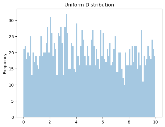
均匀分布 Uniform

数据在给定范围内（low, high）连续均匀分布

N = 2000

d = dist.Uniform(0., 10)
x = d.sample([N])
plt.hist(x, bins=100, alpha=0.4)

plt.gca().set(title='Uniform Distribution', ylabel='Frequency');
# plt.legend();

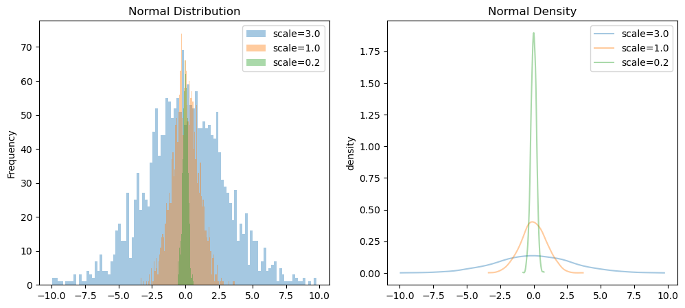
正态分布（高斯分布） Normal

正态分布，也称“常态分布”，又名高斯分布，正态曲线呈钟型，两头低，中间高，左右对称因其曲线呈钟形，因此人们又经常称之为钟形曲线。

正态分布的概率密度函数是：

\begin{equation} f(x) = \frac {e^- \frac{(x-\mu)^2}{2\sigma^2} }{\sqrt {2\pi} \sigma} \end{equation}

其中 \(\mu\) 和 \(\sigma\) 表示正态分布的位置和标准差， 当 \(\mu\)=0、\(\sigma\) =1 时称为标准正态分布；在python中经常用 loc、 std 或 mean、scale表示。

在一个标准正态分布中，约有 68.2% 的点落在 ±1 个标准差的范围内。约有 95.5% 的点落在 ±2 个标准差的范围内。约有 99.7% 的点落在 ±3 个标准差的范围内。

fig,ax=plt.subplots(ncols=2, figsize=(12, 5))

N = 2000
for s in [3.0, 1.0, 0.2]:
    d=dist.Normal(loc=0., scale=s)
    x = d.sample([N])
    ax[0].hist(x, bins=100, alpha=0.4, label=f'scale={s}')

    kde=gaussian_kde(x)
    dx=torch.linspace(x.min(),x.max(), 50)
    dy=kde(dx)
    ax[1].plot(dx,dy, alpha=0.4, label=f'scale={s}')

ax[0].set(title='Normal Distribution', ylabel='Frequency')
ax[0].legend()
ax[1].set(title='Normal Density', ylabel='density')
ax[1].legend();

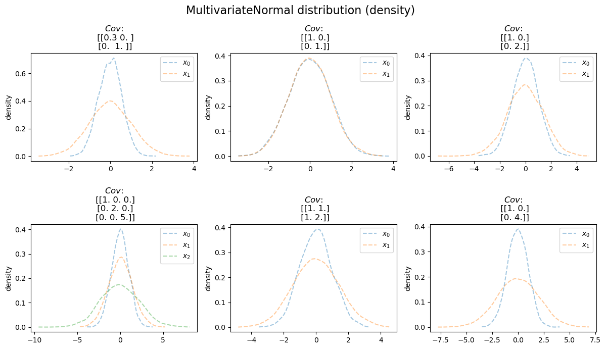
多元正态分布 Multivariate normal

多元正态分布是一元（univariate）正态分布在多维空间的扩展,即将 \(X\) 从 1 维扩展到 k 维的列向量 \(X=(X_1,X_2,\cdots,X_k)^T\) 。

多元正态分布的密度函数： \begin{equation} \begin{aligned} f(x) &= \frac{1}{\sqrt{(2\pi)^k \det\sum }} e^{ -\frac{1}{2}(x-\mu)^T \sum^{-1}(x-\mu)} \\ 其中：\\ &\mu =E(X) =(\mu_1,\mu_2,\dotsb,\mu_k) \\ \\ &\sum_{ij}=Cov(X_i,X_j) \\ \\ &\det\sum 表示协方差矩阵的行列式（determinant) \end{aligned} \end{equation}

fig, ax=plt.subplots(ncols=3, nrows=2, figsize=(12, 7))

N = 5000
covariance_matrix  = [
    np.diag([0.3,1.0]),
    np.diag([1.0,1.0]),
    np.diag([1.0,2.0]),
    np.diag([1.0,2.0,5.0]),
    np.array([ [1.0,1.0], [1.0,2.0] ]),
    np.array([ [1.0,0.0], [0.0,4.0] ]),
]

for i,s in enumerate(covariance_matrix):
    n_vars=s.shape[0]
    d=dist.MultivariateNormal(torch.zeros(n_vars), torch.tensor(s, dtype=torch.float))
    xa = d.sample([N])

    a=ax[i//3][i%3]
    # a2=a.twinx()
    # a2.set_ylabel('density');

    for j in range(len(s)):
        x=xa[:,j]
        kde=gaussian_kde(x)
        dx=torch.linspace(x.min(),x.max(), 50)
        dy=kde(dx)

        # a.hist(x, bins=100, alpha=0.2)
        a.plot(dx,dy,  '--',alpha=0.4, label=f'$x_{j}$')
    a.set(title=f'$Cov$:\n {s}', ylabel='density')
    a.legend()

fig.suptitle('MultivariateNormal distribution (density)', fontsize=16)
fig.tight_layout(h_pad=2)
plt.show()

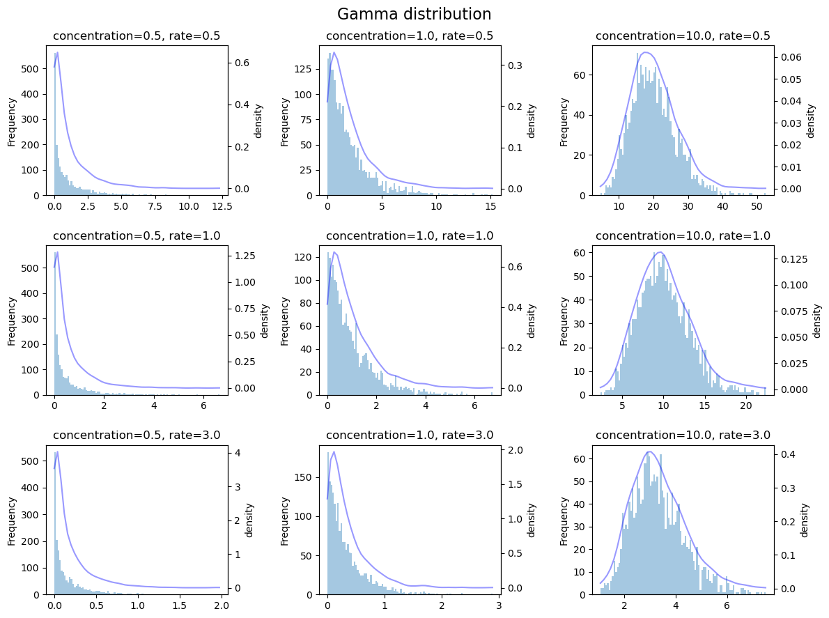
Gamma 分布

Gamma 函数的定义： \begin{equation} \begin{aligned} \Gamma(x) &=\int_0^{\infty}t^{x-1}e^{-t}dt \end{aligned} \end{equation}

Gamma 函数的重要性质：

\begin{equation} \begin{aligned} \Gamma(x+1) &= x \Gamma(x) \\ \Gamma(n) &= (n-1)! \\ \Gamma(0) &= 1 \\ \Gamma({1\over 2}) &= 2\int_0^{+\infty}e^{-u^2}du = \sqrt\pi \\ \end{aligned} \end{equation}

Gamma 分布的概率密度函数是：

\begin{equation} \begin{aligned} f(x,\alpha) = \begin{cases} \frac{x^{\alpha-1}e^{-x}}{\Gamma(\alpha)} &\text{if } x=0, \alpha>0 \\ 0 &\text{if } x<=0, \alpha>0 \end{cases} \end{aligned} \end{equation}

其中 \(\alpha\) 是形状参数。

有时，通过两个参数对Gamma分布进行参数化，此时Gamma分布的概率密度函数表示为：

\begin{equation} \begin{aligned} f(x,\alpha,\beta) = \begin{cases} \frac{\beta^\alpha x^{\alpha-1}e^{-\beta x}}{\Gamma(\alpha)}, &\text{if } x>=0, \alpha>0 \\ 0, &\text{if } x<=0, \alpha>0 \end{cases} \end{aligned} \end{equation}

fig, ax=plt.subplots(nrows=3, ncols=3, figsize=(12, 9))

N = 2000
concentrations = [0.5, 1.0, 10.0]
rates = [0.5, 1.0, 3.0]

for i,(c,r) in enumerate(product(concentrations,rates)):
    d=dist.Gamma(torch.tensor([c]), torch.tensor([r]))
    x = d.sample([N]).squeeze()

    kde=gaussian_kde(x)
    dx=torch.linspace(x.min(),x.max(), 50)
    dy=kde(dx)

    a=ax[i%3][i//3]
    a.hist(x, bins=100, alpha=0.4)
    a2=a.twinx()
    a2.plot(dx,dy, 'b-', alpha=0.4)
    a.set(title=f'concentration={c}, rate={r}', ylabel='Frequency')
    a2.set_ylabel('density');

fig.suptitle('Gamma distribution', fontsize=16)
fig.tight_layout(h_pad=2)
plt.show()

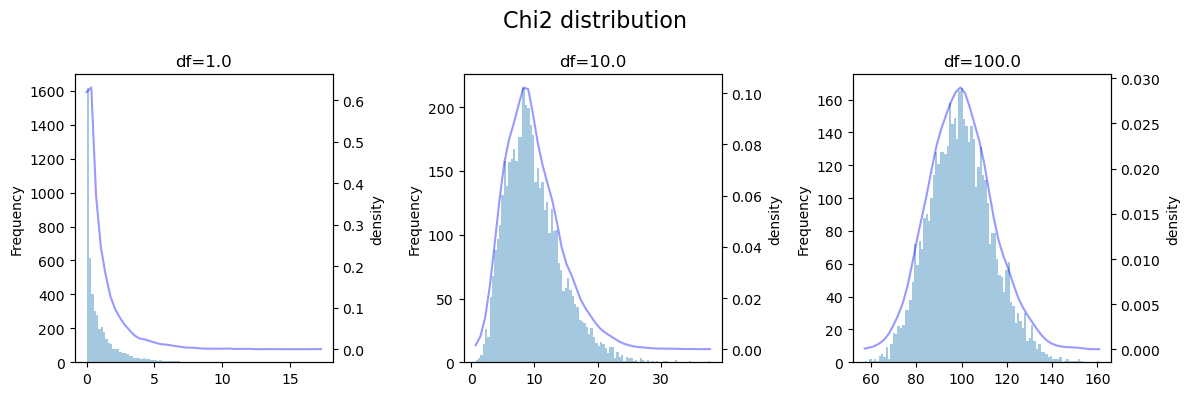
卡方分布 Chi-squared / Chi2

若 n个相互独立的随机变量1 , 2, …， n , 均服从标准正态分布（也称独立同分布于标准正态分布） ，则这 n 个服从标准正态分布的随机变量的平方和构成—新的随机变量，其分布规律称为卡方分布。

卡方分布的概率密度函数：

\begin{equation} \begin{aligned} f(x;v) &= \frac{1}{ 2^{v/2}\Gamma(v/2) } x^{v/2-1} e^{-x/2} \\ &其中: x>0, v>0 \end{aligned} \end{equation}

其中 \(v\) 是自由度（python中一般标记为df）。

卡方分布也可看作是Gamma 分布的一种特殊形式， 其中 \(a=df / 2, loc=0, scale=2\) 。

fig, ax=plt.subplots(ncols=3, figsize=(12, 4))

N = 5000
dfs = [1.0, 10.0, 100.]
for i,s in enumerate(dfs):
    d=dist.Chi2(df=torch.tensor(s))
    x = d.sample([N]).squeeze()

    kde=gaussian_kde(x)
    dx=torch.linspace(x.min(),x.max(), 50)
    dy=kde(dx)

    a=ax[i]
    a.hist(x, bins=100, alpha=0.4)
    a.set(title=f'df={s}', ylabel='Frequency')
    a2=a.twinx()
    a2.plot(dx,dy, 'b-', alpha=0.4)
    a2.set_ylabel('density');

fig.suptitle('Chi2 distribution', fontsize=16)
fig.tight_layout(h_pad=2)
plt.show()

Beta 分布

Beta分布的概率密度函数：

\begin{equation} \begin{aligned} f(x,\alpha,\beta) = \frac{\Gamma(\alpha+\beta) x^{\alpha-1} (1-x)^{\beta-1}} {\Gamma\alpha \Gamma\beta} \end{aligned} \end{equation}

其中： \(0<=x<=1, \alpha>0, \beta>0\) 。

fig, ax=plt.subplots(nrows=3, ncols=3, figsize=(12, 9))

N = 5000
concentrations0 = [0.5, 1.0, 3.0]
concentrations1 = [0.5, 1.0, 3.0]

for i,(c0,c1) in enumerate(product(concentrations0,concentrations1)):
    d=dist.Beta(torch.tensor([c0]), torch.tensor([c1]))
    x = d.sample([N]).squeeze()

    kde=gaussian_kde(x)
    dx=torch.linspace(x.min(),x.max(), 50)
    dy=kde(dx)

    a=ax[i%3][i//3]
    a.hist(x, bins=100, alpha=0.4)
    a2=a.twinx()
    a2.plot(dx,dy, 'b-', alpha=0.4)
    a.set(title=f'concentration 0/1={c0}/{c1}', ylabel='Frequency')
    a2.set_ylabel('density');

fig.suptitle('Beta distribution', fontsize=16)
fig.tight_layout(h_pad=2)
plt.show()

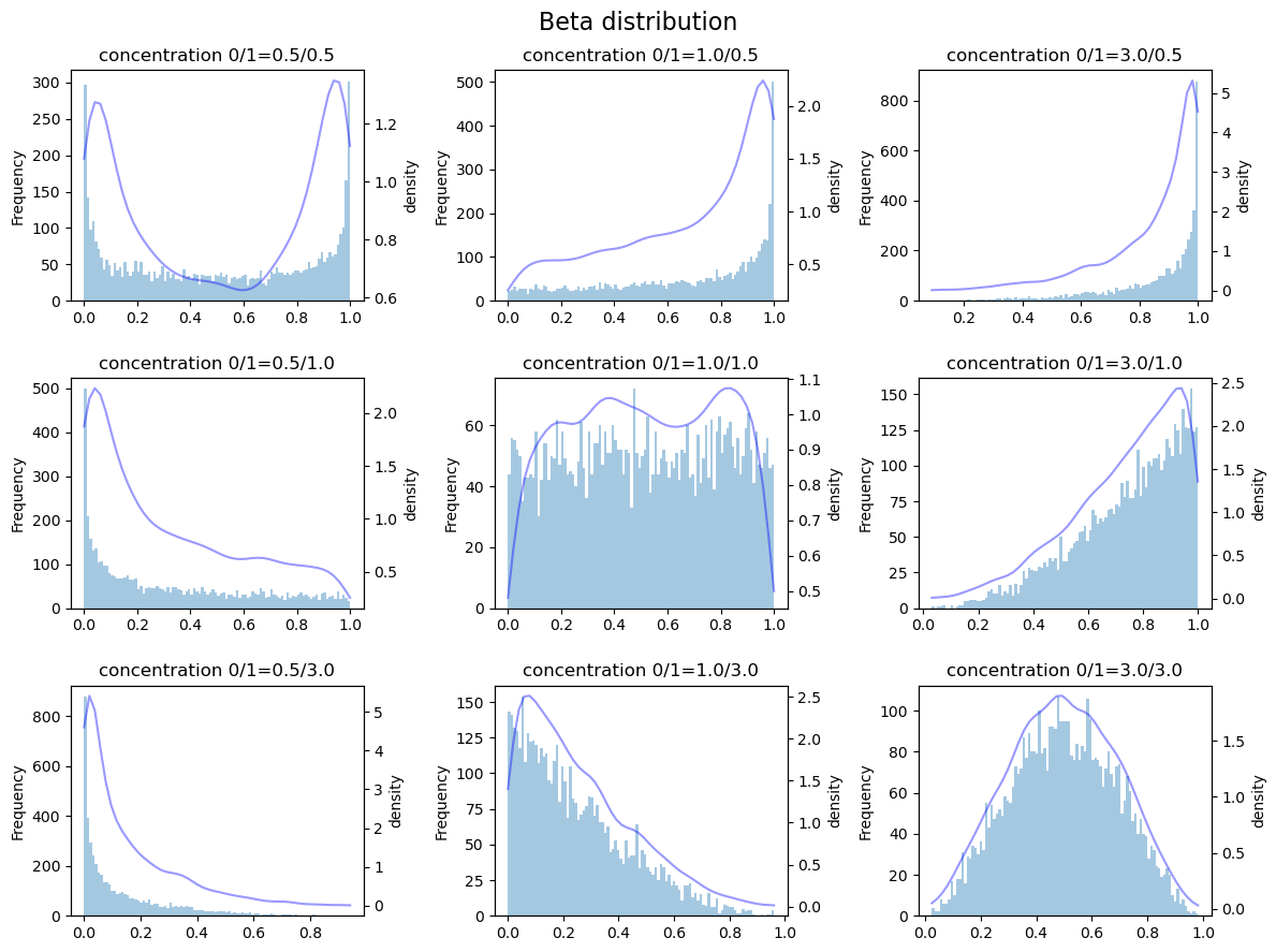
从分布图中可以看出，\(concentration<1\) 时， 数据向两侧分布；当 \(concentration==1\) 时，数据在中部的分布类似于均匀分布；\(concentration>1\) 时，数据分布类似于正态分布。

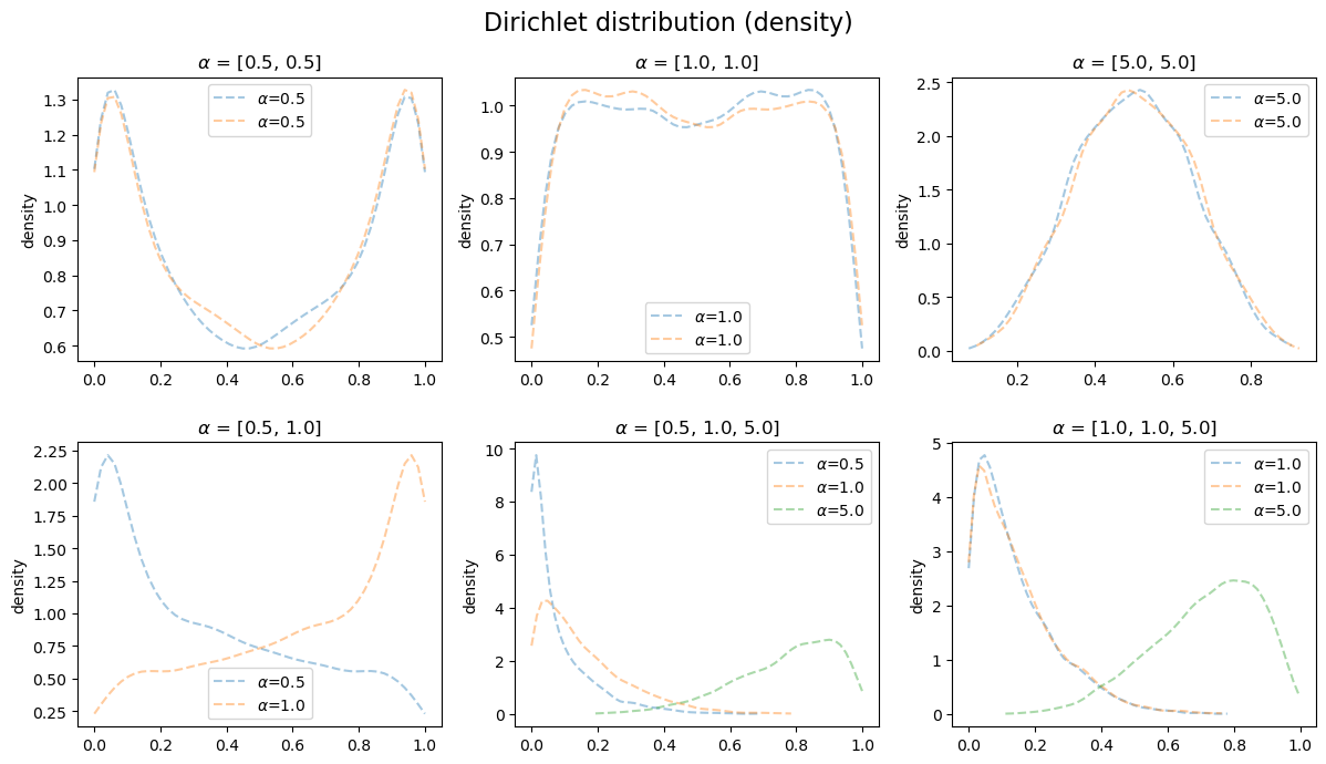
狄利克雷分布 Dirichlet

狄利克雷分布，又称多元Beta分布，是一类在实数域以正单纯形(standard simplex)为支撑集(support)的高维连续分布，是Beta分布在高维情形的推广。在Bayesian inference里，Dirichlet分布是多项分布的共轭先验。

密度函数：

\begin{equation} \begin{aligned} f(x; \alpha) &= \frac{1}{ B(\alpha)} \prod_{i=1}^K x_i ^ {\alpha_i-1} , 0 \lt x \lt 1, \alpha =(\alpha_1, ..., \alpha_K)\\ \\ where: B(\alpha) &= \frac {\prod_{i=1}^K \Gamma(\alpha_i) }{ \Gamma(\sum_{i=1}^k \alpha_i) } \end{aligned} \end{equation}

fig, ax=plt.subplots(ncols=3, nrows=2, figsize=(12, 7))

N = 5000
concentrations  = [[0.5,0.5],
                   [1.0,1.0],
                   [5.0,5.0],
                   [0.5, 1.0],
                   [0.5, 1.0, 5.0],
                   [1.0, 1.0, 5.0]]
for i,s in enumerate(concentrations):
    d=dist.Dirichlet(torch.tensor(s))
    xa = d.sample([N])

    a=ax[i//3][i%3]
    # a2=a.twinx()
    # a2.set_ylabel('density');

    for j in range(len(s)):
        x=xa[:,j]
        kde=gaussian_kde(x)
        dx=torch.linspace(x.min(),x.max(), 50)
        dy=kde(dx)

        # a.hist(x, bins=100, alpha=0.2)
        a.plot(dx,dy,  '--',alpha=0.4, label=f'$\\alpha$={s[j]}')
    a.set(title=f'$\\alpha$ = {s}', ylabel='density')
    a.legend()

fig.suptitle('Dirichlet distribution (density)', fontsize=16)
fig.tight_layout(h_pad=2)
plt.show()

拉普拉斯分布 Laplace

拉普拉斯分布的密度函数：

\begin{equation} \begin{aligned} f(x) = \frac{1}{2 \lambda} e ^ { - \frac{\vert x-\mu \vert}{\lambda} } \end{aligned} \end{equation}

当 \(\mu=0\)时：

\begin{equation} \begin{aligned} f(x) = \frac{1}{2 \lambda} e ^ { - \frac{\vert x \vert}{\lambda} } \end{aligned} \end{equation}

它是由两个指数函数组成的，所以又叫做双指数函数分布。

fig, ax=plt.subplots(ncols=3, figsize=(12, 4))

N = 5000
scales = [0.5, 1.0, 3.0]
for i,s in enumerate(scales):
    d=dist.Laplace(loc=0.0, scale=torch.tensor(s))
    x = d.sample([N]).squeeze()

    kde=gaussian_kde(x)
    dx=torch.linspace(x.min(),x.max(), 50)
    dy=kde(dx)

    a=ax[i]
    a.hist(x, bins=100, alpha=0.4)
    a2=a.twinx()
    a2.plot(dx,dy, 'b-', alpha=0.4)
    a.set(title=f'scale={s}', ylabel='Frequency')
    a2.set_ylabel('density');

fig.suptitle('Laplace distribution', fontsize=16)
fig.tight_layout(h_pad=2)
plt.show()

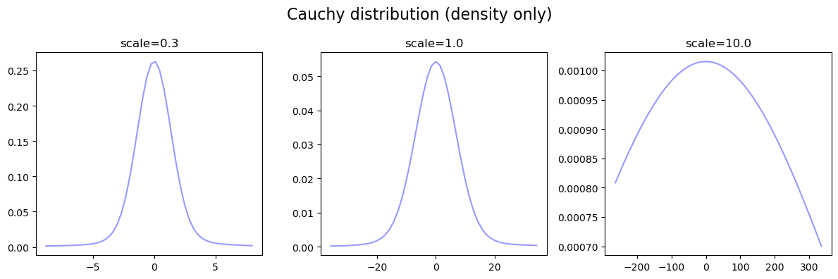
柯西分布 Cauchy

柯西分布的概率密度函数：

\begin{equation} \begin{aligned} f(x) = \frac{1}{\pi (1+x^2)} \end{aligned} \end{equation}

from scipy.stats import cauchy

fig, ax=plt.subplots(ncols=3, figsize=(12, 4))

N = 5000
scales = [0.3, 1.0, 10.0]
for i,s in enumerate(scales):
    d=dist.Cauchy(loc=0.0, scale=torch.tensor(s))
    x = d.sample([N]).squeeze()

    kde=gaussian_kde(x)
    xleft,xright = torch.quantile(x,0.01),torch.quantile(x,0.99)  #说明： 柯西分布随机数中两端离群值距离中心太远，所以在绘图时将其丢弃
    dx=torch.linspace(xleft,xright,50)
    dy=kde(dx)

    a=ax[i]
    # a.hist(x, bins=100, alpha=0.4)
    # a.set(title=f'scale={s}', ylabel='Frequency')
    # a.set_xlim(left=xleft,right=xright)
    # a2=a.twinx()
    a.plot(dx,dy, 'b-', alpha=0.4)
    a.set(title=f'scale={s}')

fig.suptitle('Cauchy distribution (density only)', fontsize=16)
fig.tight_layout(h_pad=2)
plt.show()

T分布 StudentT

T分布的概率密度函数：

\begin{equation} \begin{aligned} f(x;v) = \frac {\Gamma(\frac{v+1}{2}) }{ \sqrt{\pi v} \Gamma(\frac{v}{2}) } ( 1 + \frac{x^2}{v} )^{ - \frac{v+1}{2}} \end{aligned} \end{equation}

其中 \(v\) 是自由度（python中一般标记为df）。

特别地，当 \(v=1\) 时，T分布就是柯西分布；当 \(v \rightarrow \infty\) 时，T分布就是正态分布。

fig, ax=plt.subplots(ncols=3, figsize=(12, 4))

N = 5000
dfs = [1.0, 10.0, 100.]
for i,s in enumerate(dfs):
    d=dist.StudentT(df=torch.tensor(s))
    x = d.sample([N]).squeeze()

    kde=gaussian_kde(x)
    dx=torch.linspace(x.min(),x.max(), 50)
    dy=kde(dx)

    a=ax[i]
    a.hist(x, bins=100, alpha=0.4)
    a.set(title=f'df={s}', ylabel='Frequency')
    a2=a.twinx()
    a2.plot(dx,dy, 'b-', alpha=0.4)
    a2.set_ylabel('density');

fig.suptitle('StudentT distribution', fontsize=16)
fig.tight_layout(h_pad=2)
plt.show()

离散变量分布

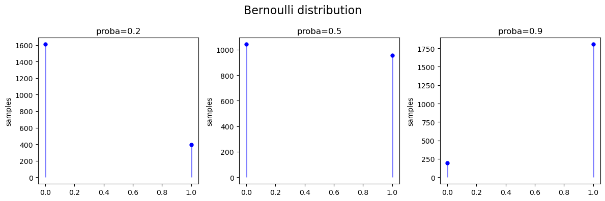
伯努利分布 Bernoulli

伯努利分布只有 成功（值为1 ) 或 失败（值为O) 这两种结果，也称为两点分布或者0-1分布，是最简单的离散型概率分布。

伯努利分布的概率质量函数：

\begin{equation} \begin{aligned} f(k) &= \begin{cases} 1-p & \text {if } k=0 \\ p & \text {if } k=1 \\ \end{cases} \\ 其中： & k \in \{0,1\}, p 是成功概率 \end{aligned} \end{equation}

fig, ax=plt.subplots(ncols=3, figsize=(12, 4))

N = 2000
probs = [0.2, 0.5, 0.9]
for i, p in enumerate(probs):
    d=dist.Bernoulli (torch.tensor(p))
    samples = d.sample([N])
    x,y = samples.unique(return_counts=True)

    a=ax[i]
    a.plot(x, y, 'bo', ms=5, label='binom pmf')
    a.vlines(x, ymin=0, ymax=y,  colors='b', lw=2, alpha=0.5)
    a.set(title=f'proba={p}', ylabel='samples')

fig.suptitle('Bernoulli distribution', fontsize=16)
fig.tight_layout(h_pad=2)
plt.show()

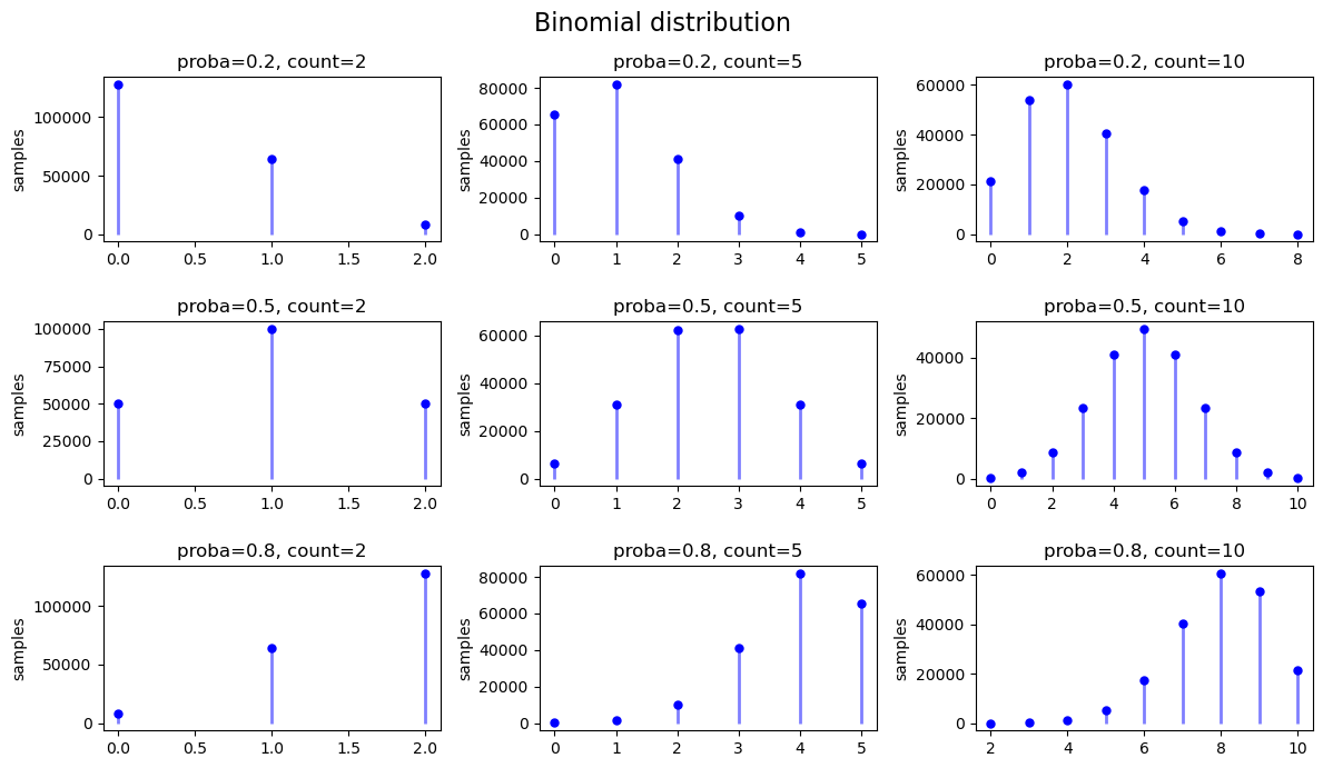
二项分布 Binomial

在 n 次独立重复的伯努利试验中，设每次试验中事件A发生的概率为p。用X表示n重伯努利试验中事件A发生的次数，则X的可能取值为0，1，…，n,且对每一个k（0≤k≤n）,事件{X=k}即为“n次试验中事件A恰好发生k次”，随机变量X的离散概率分布即为二项分布（Binomial Distribution）。

二项分布的质量函数：

\begin{equation} \begin{aligned} f(k) &= \binom{n}{k} p^k (1-p)^{n-k} \\ 其中： \\ & k \in \{0,1,...,n\}, 0 \le p \lt 1 \\ & \binom{n}{k} = \frac{n!}{k! (n-1)!}是二项式系数 \end{aligned} \end{equation}

当n=1时，二项分布就是伯努利分布。

fig, ax=plt.subplots(ncols=3, nrows=3, figsize=(12, 7))

N = 200000
probs = [0.2, 0.5,.8]
counts = [2, 5, 10]

for i, (p,c) in enumerate(product(probs,counts)):
    d=dist.Binomial(torch.tensor(c),torch.tensor(p))
    samples = d.sample([N])
    x,y = samples.unique(return_counts=True)

    a=ax[i//3][i%3]
    a.plot(x, y, 'bo', ms=5, label='binom pmf')
    a.vlines(x, ymin=0, ymax=y,  colors='b', lw=2, alpha=0.5)
    a.set(title=f'proba={p}, count={c}', ylabel='samples')

fig.suptitle('Binomial distribution', fontsize=16)
fig.tight_layout(h_pad=2)
plt.show()

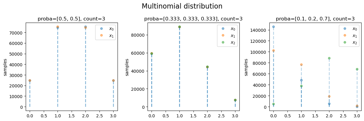
多项分布 multinomial

多项分布是二项分布的推广，即每次独立事件A不只是0和1两种结果，而是多种结果，比如投掷骰子有6种结果。

在 n 次独立重复的随机试验中，设每次试验中事件 \(A\) 有 \(k\) 种结果 \(A_1,\dotsb,A_k\), 分别将他们的出现次数记为随机变量 \(X_i,\dotsb,X_k\)，他们的概率分布是\(p_1,\dotsb,p_k\)。那么那么在n次采样的总结果中，\(A_1\) 出现 \(n_1\) 次、\(A_2\) 出现 \(n_2\)次、…、\(A_k\) 出现 \(n_k\) 次的这种事件的出现概率就是多项分布 multinomial distribution。

多项分布的质量函数：

\begin{equation} \begin{aligned} f(x) &= \frac{n!}{x_1! \dotsb x_k!} p_1^{X_1} \dotsb p_k^{X_k} \\ 其中： \\ & x_i 是非负整数且其和为 n \end{aligned} \end{equation}

fig, ax=plt.subplots(ncols=3, nrows=1, figsize=(12, 4))

N = 200000
probs = [[0.5, 0.5],
         [0.333, 0.333, 0.333],
         [0.1, 0.2, 0.7],
        ]
counts = [3,]

for i, (p,c) in enumerate(product(probs,counts)):
    d=dist.Multinomial(c,torch.tensor(p))
    samples = d.sample([N])

    a=ax[i]
    for j in range(len(p)):
        samples_j = samples[:,j]
        x,y = samples_j.unique(return_counts=True)

        a.plot(x, y, 'o', ms=5, label=f'$x_{j}$', alpha=0.5)
        a.vlines(x, ymin=0, ymax=y, linestyles='dashed', lw=2, alpha=0.3)
    a.set(title=f'proba={p}, count={c}', ylabel='samples')
    a.legend()

fig.suptitle('Multinomial distribution', fontsize=16)
fig.tight_layout(h_pad=2)
plt.show()

泊松分布 Poisson

泊松概率分布考虑的是在连续时间或空间单位上发生随机事件次数的概率， 可以看作是二项式分布的极限。

泊松分布的概率质量函数：

\begin{equation} \begin{aligned} f(k) &= \frac {e^{-\mu} \mu^k }{ k! } \\ 其中： & k \in \{0,1, ..., n\} \end{aligned} \end{equation}

fig, ax=plt.subplots(ncols=3, nrows=2, figsize=(12, 7))

N = 200000
probs = [0.2, 0.5, 1.0, 2.0, 5.0, 10.0]
for i, p in enumerate(probs):
    d=dist.Poisson (torch.tensor(p))
    samples = d.sample([N])
    x,y = samples.unique(return_counts=True)

    a=ax[i//3][i%3]
    a.plot(x, y, 'bo', ms=5, label='binom pmf')
    a.vlines(x, ymin=0, ymax=y,  colors='b', lw=2, alpha=0.5)
    a.set(title=f'$\mu$ ={p}', ylabel='samples')

fig.suptitle('Poisson distribution', fontsize=16)
fig.tight_layout(h_pad=2)
plt.show()